For my masters research, I needed a fully delineated stream network map of the Great Miami River Watershed that included all first order streams. Because of this requirement, all of the available datasets (USGS, Miami Conservancy District, etc.) were not available at the required detail level. Hence, I had to build my own map. This is a fairly common procedure, and you can actually find quite a few tutorials on it online. However, I had to look at multiple tutorials to piece together what to do. Even then, I had questions that weren’t fully satisfied until I did additional research. So here’s a step by step, with some questions answered.

First off, I highly recommend the use of the WhiteboxTools. It is available for Windows, MacOS, and Linux. While a standalone GUI is available, called the Whitebox Geospatial Analysis Tools, I recommend the use of WhiteboxTools. They can be implemented through QGIS, ArcMap, R, or Python. For the purposes of this tutorial, I will use WhiteboxTools implemented through QGIS. This flow would also work with the hydrology tools in Arc, but as an advocate for free and open source software (FOSS), I highly recommend WhiteboxTools.

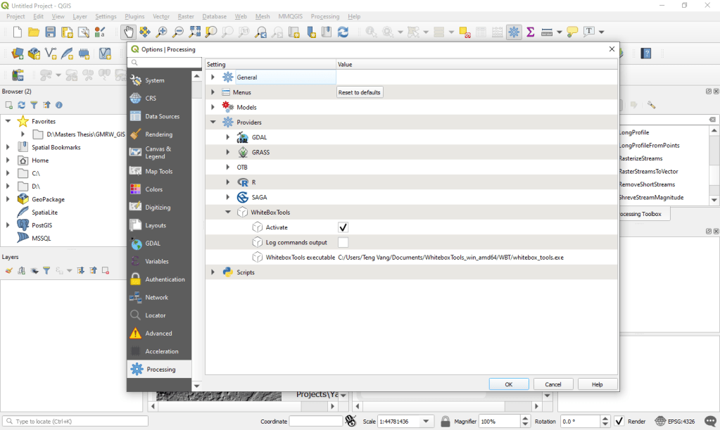
The first step is installation. Unless you plan on using the GUI, you need to make sure that you download the WhiteboxTools. I typically save it in my Documents folder. You just need to remember where you downloaded and unzipped it, as you’ll need to know it later. If you want a more detailed version of the installation instructions, you can look at the manual. For QGIS, you’ll need a plugin called Whitebox for Processing. Please note, you’ll need QGIS 3.8 or higher. The plugin is regularly updated, as I originally did all this analysis on QGIS 3.4. To install the plugin, you’ll need to add Alex’s custom repository by adding this url, https://plugins.bruy.me/plugins/plugins.xml . Please note, you’ll need to activate the plugin and add the address to the WhiteboxTools executable. To access this, click Settings -> Options -> Processing -> Providers -> WhiteboxTools. Make sure the activate checkbox is checked, and direct the executable to whitebox_tools.exe. My path is C:/…/Documents/WhiteboxTools_win_amd64/WBT/whitebox_tools.exe

Alright, ideally everything installed properly. Double check the manual first if you run into any problems. The only source data you’ll need for this is a DEM of the study area. Please note, if you’re interested in stream order, you should have a DEM of the entire watershed. DEMs can be sourced at USGS Earth Explorer or Google Earth Engine. I had great results with a 10 meter spatial resolution and would recommend that as a starting point if you’re unsure as to what spatial resolution you would like. Additionally, if you’re interested in something like stream order, you’ll need to make sure you download the DEM of the entire watershed and merge them. And if I remember correctly WhiteboxTools is partial to GeoTiffs.

First things first. There are errors with your DEM. Those errors need to be fixed. Fortunately for you, there is a tool that can take care of that. Its called BreachDepressions. However, I personally prefer another tool. Its called the FlowAccumulationFullWorkflow. The reason I prefer this tool is because it combines multiple tools into one. Since we’re interested in building a delineated stream network, its just faster to jump to this tool. This is the tool as it appears in QGIS 3.8.

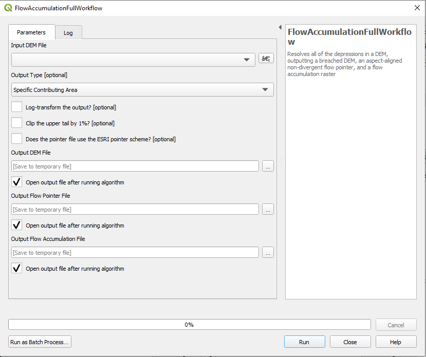
The Input DEM file is the DEM that you downloaded from Earth Explorer or Earth Engine. When in doubt, leave all the default options on. Please note, this tool will create three raster files. You’ll want to know which file is which, so make sure that you name them appropriately. Even if you’re in the ESRI ecosystem, I would recommend leaving the ESRI pointer scheme unchecked.

If you’re want stream order information or would like to know the watershed boundaries, run the basin tool. Otherwise, onto the stream extraction. You’ll need to use the ExtractStreams tool. Here’s where the guesswork is involved. You’ll notice that there’s a parameter called the channelization threshold (circled in blue below).

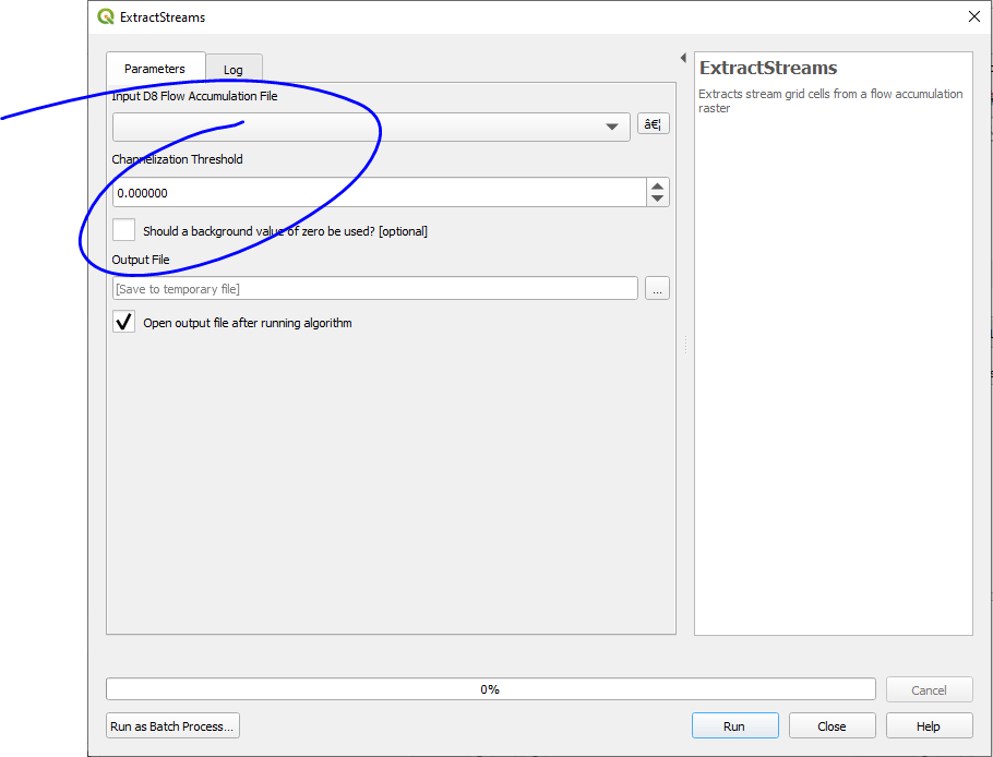
So what is the correct channelization threshold? It all depends. There’s no tool or formula for you to run to determine the correct threshold. Its one part science, one part art, and one part luck. Here’s what I recommend. Pick a value. Depending on the area that the DEM encompasses, you may need to zoom in in order to see the streams. Please note, this tool creates a raster. We’ll convert it into a vector file in a little bit. Keep in mind, the streams are also not necessarily perennial. When in doubt, vectorize the raster, place it in a GPS unit, and go check out the streams that you delineated. Yeah, I know, this probably isn’t the answer you’re looking for. You were probably hoping for something like, divide by 2 add 7. Unfortunately, this is what it is.

Alright, final step is to turn it into a vector file. You want the RasterStreamstoVector tool. And there you go, a delineated stream network. Perhaps in the future I’ll write an R script for the process. Please note, at this time, the R package is a wrapper for the Python tool and does not recognize spatial objects and simple features.

The feature image was taken by Joao Branco and is available on Unsplash.