The local convex hull method of home range estimation is a relatively recent technique. It was developed in 2004 by Getz and Wilmers. You can read the paper here and the follow up 2007 paper here. The strength of the local convex hull method, or LoCoH for short, is that it takes into account the topography of your study area. Unfortuantely, you will need a high sampling rate in order for LoCoH to properly model your home range. So if all you have is resight data, e.g. less than 30 points, LoCoH probably isn’t for you. Consider KDE instead. You’ll need data along the lines of that obtained by GPS tags/collars sampled at least a couple times a day for an accurate result.

There are three LoCoH methods. If you review the documentation for adehabitatHR, there’s a tutorial for k-LoCoH. Here, I’ll review how I use a-LoCoH. a-LoCoH, or adaptive radius LoCoH, is a hybridization of k-LoCoH and r-LoCoH. a-LoCoH is considered the best one to use (Getz et al 2007), but its up to you to determine which one you prefer for your study.

As with kernel density estimates, your CSV file of coordinates should be in UTM format. If it isn’t in UTM format, then you’ll need to transform it. There are two ways that you can do this depending on what you’re comfortable with. Please refer to my blog post here for more detailed directions.

While I do plan to create an ArcGIS plugin eventually using Python, I haven’t gotten around to it just yet. When I do, I’ll update this post with the appropriate information. Please note, this method requires R and the adehabitatHR package. If you wish to export the shapefile for use within GIS software, you’ll also need the rgdal and sp packages.

Perhaps the most time consuming aspect for a-LoCoH is to get the parameter correct. I hate to say it, but there is some subjectivity in this area. You can review the papers to see how the authors address this, but suffice it to say that it is not a huge issue and LoCoH is used quite often in the home range literature. Until I have a working plugin for ArcGIS, here’s the trick I use to get a feel for the parameter. I use the OpenJUMP HoRAE package. To read more about OpenJUMP, please visit their website. To read more about HoRAE, please refer to their website and their wikipage.

Before we begin discussing the technical details, you might be asking me, Teng, why don’t I just use the HoRAE package instead of using R? That is a very good question. First off, if your coordinates aren’t in UTM notation, I’m not sure how to convert it into UTM using HoRAE. Secondly, there are limitations to HoRAE. You can customize the percent contours you want using R. There are preset values in HoRAE, so you may not necessarily get the percent contour you want. For example, if you’re looking for the 95% contour in HoRAE, you won’t be able to calculate it. At least not for LoCoH. However, it is useful in terms of modeling the parameter. Please note, I am not an avid OpenJUMP user, so I will not be able to provide much technical support for you. It is a tool I use strictly for one thing. If you’re not comfortable working with command line, it may be a tool you wish to become familiar with. The documentation is quite good for HoRAE, and in my opinion, something a novice could easily follow.

When determining the parameter, you’ll need to consider the minimum spurious holes rule. Getz and Wilmers 2004 define it as “the smallest value that produces a covering that has the same topology as the given set.” The paper goes into more detail, but basically you need to select a parameter thats big enough so that your home range doesn’t look like swiss cheese, but small enough that lakes, cliffs, etc. aren’t included in your analysis. But where do you even start? So this isn’t a hard fast rule, but for me, I normally begin by considering the distance between your two furthest points. For example, if its 10,000 meters, then I would start with 10,000 for your parameter and adjust from there.

Here is an example of a parameter that is too small. Please note the swiss cheese effect.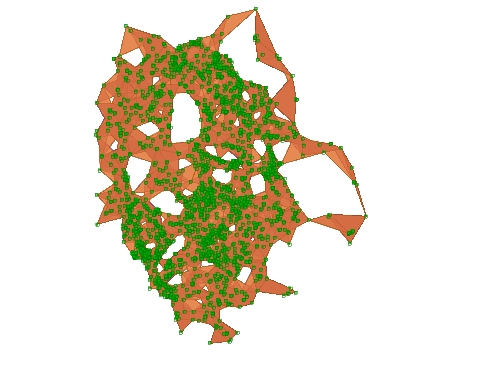

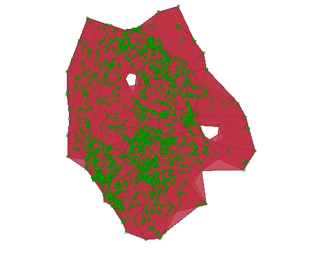
Using the same dataset, here is an example of an appropriate parameter being selected.

A common problem is what is called the donut hole. When you’re getting close to an appropriate parameter, you’ll have a donut hole in the center. Unless there’s a specific reason for why your study animal(s) wouldn’t enter the donut hole, e.g. a lake, then you need to cover it up. Here is an example of a donut hole using the same data set.

Unfortunately, using a-LoCoH, and unlike k-LoCoH, there’s no current hard rule to determine the parameter. As a friend once told me, you need to model it until it looks right. It sounds pretty unscientific, but weirdly enough, its a good rule of thumb.

Once you’ve determined the parameter you would like to use, then its time to jump over into R. Here’s the script that I use. As a reminder, if you need to install the packages, use the install.packages() function.

> library(adehabitatHR)
> library(rgdal)
> library(sp)

> coords = read.csv(“coords.csv”, header = TRUE) ##reminder to change the csv filename to whatever it is you are currently using
> coords.data.xy <- coords[c(“X”, “Y”)]

> coords.xy <- SpatialPoints(coords.data.xy)

> coords.area <- LoCoH.a(coords.xy, parameter, unin = c(“m”), unout = c(“m2”))

> proj4string(coords.area) <- CRS(“+init=epsg:”) ##insert your epsg code after the colon and before the quotation marks ##if you need a shapefile, run the following line of code

> writeOGR(coords.area, “.”, “Some file name here”, driver = “ESRI Shapefile”)

##if you need a percent countour, run the following line of code
##remember that units are in m^2, and you’ll need to convert units as necessary if you want km^2
##don’t forget to change the percent to whatever percent you need, e.g. 35%, 45%
> LoCoH.a.area(coords.xy, percent = 95, parameter, unin = (“m”), unout = c(“m2”)

The featured image is called LoCoH. LoCoH by Teng Keng Vang is licensed under a Creative Commons Attribution-NonCommercial 4.0 International License.