Three of the most popular methods of home range estimation right now are the minimum convex polygon (MCP), kernel density estimation (KDE), and local convex hull (LoCoH). While there are a multitude more methods out there, e.g. brownian bridges and permissible home range estimation, these are the three methods I’m most familiar with. All examples were calculated using the same data set.

Before I begin discussing the methods, it is important to note that the home range is just a hypothesis. You are basically stating, using whatever method you choose, that you believe an individual has x percent of being found within this contour.

The minimum convex polygon is the simplest method to employ. Its basically the smallest area polygon that includes all location points. An easy way to visualize it is to imagine all of your GPS points as thumbtacks on a board. Take a rubber band and place it around all your thumb tacks. The polygon that is created by the rubber band is your minimum convex polygon. In this day and age, with the tools we have, I do not recommend this method at all. However, it is still in use so I provide this just as background information.

PROS: very easy to calculate, older literature uses it making temporal comparisons possible

CONS: grossly overestimates the home range, unable to calculate isopleths/percent contours

Example of MCP:

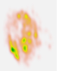
Kernel density estimation produces a density estimate based on the clustering of your GPS points. They’re able to produce estimates of any shape and size. Some of the literature indicates they overestimate the home range, while other studies show that they produce similar estimates to the next method, LoCoH. I discuss how to do kernel density estimates here.

PROS: relatively easy to calculate, very popular method in the current literature

CONS: arguably overestimate home ranges (some of the literature states no quantifiable difference whereas other articles state there is), assumes no barriers to movement

Example of KDE:

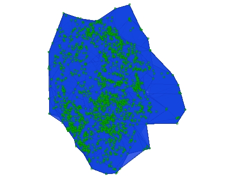
The local convex hull method works by constructing a multitude of minimum convex polygons based on a user defined parameter. The user defined parameter is guided by the minimum spurious holes covering rule. Basically, you shouldn’t have any holes in your estimate, save for those that delineate the boundaries of naturally occurring barriers. For example, if you have a puma who’s home range has a giant lake in it, its okay for there to be a hole in your home range that indicates the presence of the lake. I discuss how to calculate local convex hulls here.

PROS: takes into consideration hard boundaries, arguably more accurate than KDEs

CONS: relatively harder and longer to build, estimates may be subjective depending on parameters selected, need a large sample size of GPS points in order for it to be accurate

Example of LoCoH:

The featured image is Home, home on the range… by Johanna Madjedi used under CC 2.0.

The home range images by Teng Keng Vang is licensed under a Creative Commons Attribution-NonCommercial 4.0 International License.